|
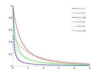
Probability density function  GPD distribution functions for and different values of and | |||
|
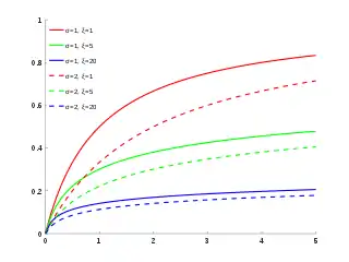
Cumulative distribution function  | |||
| Parameters | shape (real) | ||
|---|---|---|---|
| Support |
| ||
|
| |||
| CDF | |||
| Mean | |||
| Median | |||
| Mode | |||
| Variance | |||
| Skewness | |||
| Ex. kurtosis | |||
| Entropy | |||
| MGF | |||
| CF | |||
| Method of Moments |
| ||
| Expected shortfall | [1] | ||
In statistics, the generalized Pareto distribution (GPD) is a family of continuous probability distributions. It is often used to model the tails of another distribution. It is specified by three parameters: location , scale , and shape .[2][3] Sometimes it is specified by only scale and shape[4] and sometimes only by its shape parameter. Some references give the shape parameter as .[5]
Definition
The standard cumulative distribution function (cdf) of the GPD is defined by[6]
where the support is for and for . The corresponding probability density function (pdf) is
Characterization
The related location-scale family of distributions is obtained by replacing the argument z by and adjusting the support accordingly.
The cumulative distribution function of (, , and ) is
where the support of is when , and when .
The probability density function (pdf) of is
- ,
again, for when , and when .
The pdf is a solution of the following differential equation:
Special cases
- If the shape and location are both zero, the GPD is equivalent to the exponential distribution.
- With shape , the GPD is equivalent to the continuous uniform distribution .[7]
- With shape and location , the GPD is equivalent to the Pareto distribution with scale and shape .
- If , , , then . (exGPD stands for the exponentiated generalized Pareto distribution.)
- GPD is similar to the Burr distribution.
Generating generalized Pareto random variables
Generating GPD random variables
If U is uniformly distributed on (0, 1], then
and
Both formulas are obtained by inversion of the cdf.
In Matlab Statistics Toolbox, you can easily use "gprnd" command to generate generalized Pareto random numbers.
GPD as an Exponential-Gamma Mixture
A GPD random variable can also be expressed as an exponential random variable, with a Gamma distributed rate parameter.
and
then
Notice however, that since the parameters for the Gamma distribution must be greater than zero, we obtain the additional restrictions that: must be positive.
Exponentiated generalized Pareto distribution
The exponentiated generalized Pareto distribution (exGPD)

If , , , then is distributed according to the exponentiated generalized Pareto distribution, denoted by , .
The probability density function(pdf) of , is
where the support is for , and for .
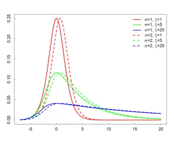
For all , the becomes the location parameter. See the right panel for the pdf when the shape is positive.
The exGPD has finite moments of all orders for all and .

The moment-generating function of is
where and denote the beta function and gamma function, respectively.
The expected value of , depends on the scale and shape parameters, while the participates through the digamma function:
Note that for a fixed value for the , the plays as the location parameter under the exponentiated generalized Pareto distribution.
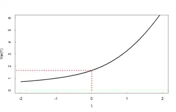
The variance of , depends on the shape parameter only through the polygamma function of order 1 (also called the trigamma function):
See the right panel for the variance as a function of . Note that .
Note that the roles of the scale parameter and the shape parameter under are separably interpretable, which may lead to a robust efficient estimation for the than using the . The roles of the two parameters are associated each other under (at least up to the second central moment); see the formula of variance wherein both parameters are participated.
The Hill's estimator
Assume that are observations (not need to be i.i.d.) from an unknown heavy-tailed distribution such that its tail distribution is regularly varying with the tail-index (hence, the corresponding shape parameter is ). To be specific, the tail distribution is described as
It is of a particular interest in the extreme value theory to estimate the shape parameter , especially when is positive (so called the heavy-tailed distribution).
Let be their conditional excess distribution function. Pickands–Balkema–de Haan theorem (Pickands, 1975; Balkema and de Haan, 1974) states that for a large class of underlying distribution functions , and large , is well approximated by the generalized Pareto distribution (GPD), which motivated Peak Over Threshold (POT) methods to estimate : the GPD plays the key role in POT approach.
A renowned estimator using the POT methodology is the Hill's estimator. Technical formulation of the Hill's estimator is as follows. For , write for the -th largest value of . Then, with this notation, the Hill's estimator (see page 190 of Reference 5 by Embrechts et al ) based on the upper order statistics is defined as
In practice, the Hill estimator is used as follows. First, calculate the estimator at each integer , and then plot the ordered pairs . Then, select from the set of Hill estimators which are roughly constant with respect to : these stable values are regarded as reasonable estimates for the shape parameter . If are i.i.d., then the Hill's estimator is a consistent estimator for the shape parameter .
Note that the Hill estimator makes a use of the log-transformation for the observations . (The Pickand's estimator also employed the log-transformation, but in a slightly different way .)
See also
References
- ↑ Norton, Matthew; Khokhlov, Valentyn; Uryasev, Stan (2019). "Calculating CVaR and bPOE for common probability distributions with application to portfolio optimization and density estimation" (PDF). Annals of Operations Research. Springer. 299 (1–2): 1281–1315. arXiv:1811.11301. doi:10.1007/s10479-019-03373-1. S2CID 254231768. Retrieved 2023-02-27.
- ↑ Coles, Stuart (2001-12-12). An Introduction to Statistical Modeling of Extreme Values. Springer. p. 75. ISBN 9781852334598.
- ↑ Dargahi-Noubary, G. R. (1989). "On tail estimation: An improved method". Mathematical Geology. 21 (8): 829–842. doi:10.1007/BF00894450. S2CID 122710961.
- ↑ Hosking, J. R. M.; Wallis, J. R. (1987). "Parameter and Quantile Estimation for the Generalized Pareto Distribution". Technometrics. 29 (3): 339–349. doi:10.2307/1269343. JSTOR 1269343.
- ↑ Davison, A. C. (1984-09-30). "Modelling Excesses over High Thresholds, with an Application". In de Oliveira, J. Tiago (ed.). Statistical Extremes and Applications. Kluwer. p. 462. ISBN 9789027718044.
- ↑ Embrechts, Paul; Klüppelberg, Claudia; Mikosch, Thomas (1997-01-01). Modelling extremal events for insurance and finance. Springer. p. 162. ISBN 9783540609315.
- ↑ Castillo, Enrique, and Ali S. Hadi. "Fitting the generalized Pareto distribution to data." Journal of the American Statistical Association 92.440 (1997): 1609-1620.
Further reading
- Pickands, James (1975). "Statistical inference using extreme order statistics" (PDF). Annals of Statistics. 3 s: 119–131. doi:10.1214/aos/1176343003.
- Balkema, A.; De Haan, Laurens (1974). "Residual life time at great age". Annals of Probability. 2 (5): 792–804. doi:10.1214/aop/1176996548.
- Lee, Seyoon; Kim, J.H.K. (2018). "Exponentiated generalized Pareto distribution:Properties and applications towards extreme value theory". Communications in Statistics - Theory and Methods. 48 (8): 1–25. arXiv:1708.01686. doi:10.1080/03610926.2018.1441418. S2CID 88514574.
- N. L. Johnson; S. Kotz; N. Balakrishnan (1994). Continuous Univariate Distributions Volume 1, second edition. New York: Wiley. ISBN 978-0-471-58495-7. Chapter 20, Section 12: Generalized Pareto Distributions.
- Barry C. Arnold (2011). "Chapter 7: Pareto and Generalized Pareto Distributions". In Duangkamon Chotikapanich (ed.). Modeling Distributions and Lorenz Curves. New York: Springer. ISBN 9780387727967.
- Arnold, B. C.; Laguna, L. (1977). On generalized Pareto distributions with applications to income data. Ames, Iowa: Iowa State University, Department of Economics.